Let’s continue our conversation on spreadsheet basics. Assuming your home care scheduling software lets you get hold of the data itself, you can use it for more in-depth, ad hoc reporting.
To see the previous article, click on Spreadsheet Basics.
In this second article we’ll touch on:
- More advanced navigation and selection options
- Hiding, showing and freezing columns
Keyboard Navigation and Selection
In the first article, we looked at the basics of navigation: clicking on cells, rows and columns, clicking & dragging to select a range and selecting the entire sheet. As you work more and more in spreadsheets, you’ll start to want some more efficient ways of selecting things. On large and complicated spreadsheets, clicking and dragging can be tedious. Happily, there are some handy tricks for navigating and selecting using the keyboard.
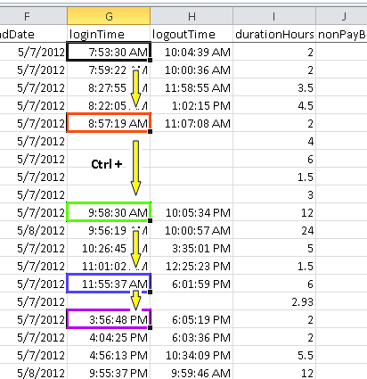 Using the arrow keys, you can move the selection from one cell to another in the direction of the arrow. If you hold the Ctrl key down while using an arrow key, something very interesting will happen: the selection will jump to the cell before the next empty cell. Hit it again and it jumps over the blank space to the next cell with content. This is very handy for finding the ‘holes’ in a column or row.
Moving the selection: effect of using Ctrl+Arrow keys (in this case, the Down Arrow key, starting with cell G2)
You can also use the arrow keys to select multiple cells. Hold the Shift key down and it will extend the selection as you tap. You can combine horizontal and vertical Arrow keys to expand (or contract) the selection in rows and columns. You can also combine the Shift and Ctrl key to ‘jump’ the selection out to the next cell before or after a blank one.
Another option to throw in is the use of the Page Up, Page Down, Home and End keys. These keys move you quickly in very specific ways.
It’s a good idea to play around with these different key combinations and get a feel for how each one works. Most of them have value in other places besides Excel. For example, Ctrl-Home is almost universally a way to get to the very beginning of a document from wherever you are.
Keeping the stuff in sight (or out of sight)
Freezing Panes
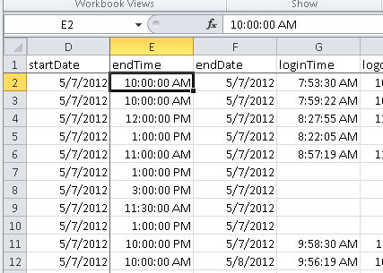 It’s worth talking a bit about arranging your spreadsheet so you can always tell where you are. In a large file, it’s easy to get confused about which column is which, if you aren’t near the top. You can ‘freeze’ the top row so it’s always visible, no matter how far down the list you might be.
To do that, go to the View tab and click on Freeze Panes, then select Freeze Top Row. Now no matter where you are in the spreadsheet, you’ll always see the column headings.
You can do a similar thing with the columns on the left, to make it clear which row you’re on. To do that, click on the first cell that is below the top row or rows you want to keep visible, and to the right of the last column you want to keep visible. Then click on View, Freeze Panes and select Freeze Panes from the menu. Now, when you scroll right, the left column(s) will remain visible and, when you scroll down, you’ll always see the top row(s).
Delete, Clear, Hide and Unhide
Often you want to focus on certain data and the rest of it is just getting in the way. You can remove or hide data in a few different ways. To remove the contents of cells (without remove the cell, column or row), just select it and hit the Delete key. If you actually want the cell (or column or row) gone, click on the Home tab, select Delete (Row, Column or Cell).
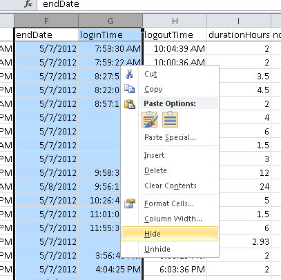
If you don’t want to get rid of the contents but simply hide them, you can do that very simply. Select the Columns or Rows (must be entire columns or rows, not just blocks of cells), then right-click anywhere on the selection. In that menu, select Hide. The rows or columns will dissappear, but they’re not really gone. You can tell because the row numbers or column letters will be skipped. For example, if you hide column C,D and E, the column headings will go A,B,F,G, etc.
To bring them back, select the columns or rows on either side of them, right-click and select Unhide.
I hope this has been helpful in your quest to gain greater understanding and control of your data. In my next article of this series, I’ll go into Filtering as well as starting to analyze your data with Pivot Tables.
As always, if you have comments I’d love to hear them, and if you’re struggling with your spreadsheets, give us a call!