This is the third in a series of articles about working with spreadsheet data. The series is intended primarily for the novice user, and it assumes that your home care scheduling software lets you get hold of the data itself for more in-depth, ad hoc reporting. Of course, these techniques can be used for any set of data, as long as it’s organized in a standard data format, with one row per entry and each column representing a different field.
In this second article we’ll touch on using Excel’s built-in filters. To see the previous articles, click on Working with Spreadsheets #1 about the basics of spreadsheets or Working with Spreadsheets #2 about navigating spreadsheets.
Filtering
In previous articles we looked at bringing order to your spreadsheet using Sorting, hiding rows & columns and other simple techniques. Another way to clarify and organize the data is by using Filtering. Filtering allows you to show and hide rows based on specific criteria.
For example, if you had a list of all your shifts for last week and you wanted to limit it to only those for certain caregivers, you could sort them and delete the ones that don’t match. Or you could use the filters. A nice thing about filters is that they don’t actually remove those that don’t match, they simply hide them. That way you can change the filter over and over as you examine different aspects of the data. This is great for brainstorming about your operations, using existing data as a starting point for learning and improving things.
Turning on Filters

Assuming you have a standard MS Office layout, you can turn filtering on from the one of two places.
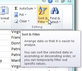
- On the Home tab, click on the Sort & Filter button on the far right and click on Filter from the drop-down menu.
- On the Data tab, click on the Filter button in the middle.
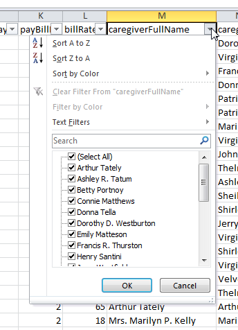
 With that done, you will notice that each column heading now has a drop-down arrow on it. In the bottom part of this dialog box, there is a list of each unique item within the column that you’ve chosen. You can pick and choose which ones are shown by checking and un-checking the boxes. The search box will let you type in all or part of a word or value to see if anything matches. You can also toggle (go back and forth) all or none from here.
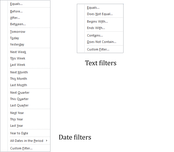
This is a very simple use of filtering. You might want to get fancier by using the advanced filters. Just above the list (mentioned above), there is a single item that will change based on the type of data in the column. If it finds text in the column, it will say ‘Text Filters’; if it’s dates, it will say ‘Date Filters’, etc.
 For example, you might to look at shifts that happened before a specific date, then look at individual caregivers within that set. To do this, use the Date Filters on the startDate column, choose Before… and set the date. It will then only show shifts that started before that date. Now you can use your drop-down filters to look at individual caregivers’ shifts in that date range.
When you want to remove a filter, click on the drop-down filter and select ‘Clear Filter From…’ If you want to get rid of all filters, just go back to the original Filter button (in theHome or Data tabs).
As usual, we’ve just touched on the basics of Filtering in Excel. As you get to know these tools, you’ll find your own uses that can dramatically improve your understanding of your data, and of your business.
Let me know if you’re finding these articles useful, or if you have suggestions or requests about them.
